library(ggplot2)
library(knitr)
library(survival)
library(survminer)
library(data.table)
df <- fread("WA_Fn-UseC_-HR-Employee-Attrition.csv")
source("custom_themes.R") # import pre-built custom themesEmployee Retention Analysis Using Survival Modeling in R (2/2)
HR analytics
Statistics
R
In the previous post, the fundamentals of survival modeling were introduced, covering how to create a survival object, fit a Kaplan-Meier model, and visualize survival curves.
This follow-up post explains how distinct values of a single variable, as well as combinations of multiple variables, can help uncover differences in retention ratios across employee cohorts.
Loading the required packages and data
Survival object creation
df[, Attrition := ifelse(Attrition == "Yes", 1, 0)]
s_obj <- Surv(time = df$YearsAtCompany, event = df$Attrition)
head(s_obj)
[1] 6 10+ 0 8+ 2+ 7+
Exploring the BusinessTravel and OverTime variables
For this exercise, the BusinessTravel and OverTime variables are examined to understand how they relate to employee retention.
kable(table(df$BusinessTravel, df$OverTime))| No | Yes | |
|---|---|---|
| Non-Travel | 115 | 35 |
| Travel_Frequently | 191 | 86 |
| Travel_Rarely | 748 | 295 |
Recoding both variables, so that the chart labels read as plain English rather than as stored values.
df[, OverTime := ifelse(OverTime == "No", "No Over Time", "Over Time")]
df[, BusinessTravel := fcase(BusinessTravel == "Non-Travel", "No travel",
                             BusinessTravel == "Travel_Rarely", "Travels rarely",
                             BusinessTravel == "Travel_Frequently", "Travels frequently")]
kable(table(df$BusinessTravel, df$OverTime))| No Over Time | Over Time | |
|---|---|---|
| No travel | 115 | 35 |
| Travels frequently | 191 | 86 |
| Travels rarely | 748 | 295 |
The table above also gives the size of each group, which is worth carrying into the last chart: the six combined groups range from 35 to 748 employees.
Fitting Kaplan-Meier models for single variables and their combinations
km_fit_BusinessTravel <- survfit(s_obj ~ BusinessTravel, data = df)
km_fit_OverTime <- survfit(s_obj ~ OverTime, data = df)
km_fit_BusinessTravel_OverTime <- survfit(s_obj ~ BusinessTravel + OverTime, data = df)
Simplifying the strata names to make interpretation easier. All three models are fitted through the data argument, so their strata are named the same way and a single expression cleans all of them.
strip_prefix <- function(fit) {
  names(fit$strata) <- gsub("BusinessTravel=|OverTime=", "", names(fit$strata))
  fit
}
km_fit_BusinessTravel <- strip_prefix(km_fit_BusinessTravel)
km_fit_OverTime <- strip_prefix(km_fit_OverTime)
km_fit_BusinessTravel_OverTime <- strip_prefix(km_fit_BusinessTravel_OverTime)
The model summaries are converted into a clean table to review the survival statistics for each group.
km_fit_summary_BusinessTravel <- as.data.table(summary(km_fit_BusinessTravel)[c("strata","time", "n.risk", "n.event", "n.censor", "surv", "std.err")])
km_fit_summary_OverTime <- as.data.table(summary(km_fit_OverTime)[c("strata","time", "n.risk", "n.event", "n.censor", "surv", "std.err")])
km_fit_summary_BusinessTravel_OverTime <- as.data.table(summary(km_fit_BusinessTravel_OverTime)[c("strata","time", "n.risk", "n.event", "n.censor", "surv", "std.err")])
NoteShow survival summary table for BusinessTravel
kable(km_fit_summary_BusinessTravel, digits = 3)| strata | time | n.risk | n.event | n.censor | surv | std.err |
|---|---|---|---|---|---|---|
| No travel | 0 | 150 | 1 | 6 | 0.993 | 0.007 |
| No travel | 1 | 143 | 4 | 14 | 0.966 | 0.015 |
| No travel | 2 | 125 | 1 | 5 | 0.958 | 0.017 |
| No travel | 3 | 119 | 1 | 15 | 0.950 | 0.019 |
| No travel | 4 | 103 | 1 | 8 | 0.941 | 0.021 |
| No travel | 5 | 94 | 2 | 19 | 0.921 | 0.024 |
| No travel | 10 | 38 | 2 | 42 | 0.872 | 0.041 |
| Travels frequently | 0 | 277 | 7 | 4 | 0.975 | 0.009 |
| Travels frequently | 1 | 266 | 17 | 8 | 0.912 | 0.017 |
| Travels frequently | 2 | 241 | 7 | 23 | 0.886 | 0.019 |
| Travels frequently | 3 | 211 | 6 | 14 | 0.861 | 0.021 |
| Travels frequently | 4 | 191 | 6 | 17 | 0.834 | 0.023 |
| Travels frequently | 5 | 168 | 4 | 22 | 0.814 | 0.025 |
| Travels frequently | 6 | 142 | 4 | 15 | 0.791 | 0.027 |
| Travels frequently | 7 | 123 | 3 | 13 | 0.772 | 0.028 |
| Travels frequently | 8 | 107 | 3 | 14 | 0.750 | 0.030 |
| Travels frequently | 9 | 90 | 2 | 17 | 0.733 | 0.032 |
| Travels frequently | 10 | 71 | 5 | 20 | 0.682 | 0.037 |
| Travels frequently | 11 | 46 | 1 | 4 | 0.667 | 0.039 |
| Travels frequently | 13 | 39 | 1 | 7 | 0.650 | 0.042 |
| Travels frequently | 18 | 26 | 1 | 11 | 0.625 | 0.047 |
| Travels frequently | 21 | 15 | 1 | 9 | 0.583 | 0.059 |
| Travels frequently | 23 | 8 | 1 | 3 | 0.510 | 0.086 |
| Travels rarely | 0 | 1043 | 8 | 18 | 0.992 | 0.003 |
| Travels rarely | 1 | 1017 | 38 | 90 | 0.955 | 0.006 |
| Travels rarely | 2 | 889 | 19 | 72 | 0.935 | 0.008 |
| Travels rarely | 3 | 798 | 13 | 79 | 0.920 | 0.009 |
| Travels rarely | 4 | 706 | 12 | 66 | 0.904 | 0.010 |
| Travels rarely | 5 | 628 | 15 | 134 | 0.882 | 0.011 |
| Travels rarely | 6 | 479 | 5 | 45 | 0.873 | 0.012 |
| Travels rarely | 7 | 429 | 8 | 60 | 0.857 | 0.013 |
| Travels rarely | 8 | 361 | 6 | 49 | 0.843 | 0.014 |
| Travels rarely | 9 | 306 | 6 | 43 | 0.826 | 0.015 |
| Travels rarely | 10 | 257 | 11 | 75 | 0.791 | 0.018 |
| Travels rarely | 11 | 171 | 1 | 20 | 0.786 | 0.018 |
| Travels rarely | 13 | 139 | 1 | 23 | 0.780 | 0.019 |
| Travels rarely | 14 | 126 | 2 | 12 | 0.768 | 0.021 |
| Travels rarely | 15 | 112 | 1 | 11 | 0.761 | 0.022 |
| Travels rarely | 16 | 100 | 1 | 10 | 0.754 | 0.023 |
| Travels rarely | 17 | 89 | 1 | 8 | 0.745 | 0.024 |
| Travels rarely | 19 | 73 | 1 | 13 | 0.735 | 0.026 |
| Travels rarely | 20 | 66 | 1 | 19 | 0.724 | 0.028 |
| Travels rarely | 22 | 37 | 1 | 20 | 0.704 | 0.033 |
| Travels rarely | 24 | 25 | 1 | 3 | 0.676 | 0.042 |
| Travels rarely | 31 | 11 | 1 | 11 | 0.615 | 0.070 |
| Travels rarely | 32 | 9 | 1 | 0 | 0.546 | 0.090 |
| Travels rarely | 33 | 8 | 1 | 2 | 0.478 | 0.101 |
| Travels rarely | 40 | 1 | 1 | 4 | 0.000 | NaN |
NoteShow survival summary table for OverTime
kable(km_fit_summary_OverTime, digits = 3)| strata | time | n.risk | n.event | n.censor | surv | std.err |
|---|---|---|---|---|---|---|
| No Over Time | 0 | 1054 | 6 | 24 | 0.994 | 0.002 |
| No Over Time | 1 | 1024 | 31 | 85 | 0.964 | 0.006 |
| No Over Time | 2 | 908 | 12 | 80 | 0.951 | 0.007 |
| No Over Time | 3 | 816 | 6 | 82 | 0.944 | 0.007 |
| No Over Time | 4 | 728 | 11 | 69 | 0.930 | 0.008 |
| No Over Time | 5 | 648 | 7 | 132 | 0.920 | 0.009 |
| No Over Time | 6 | 509 | 4 | 48 | 0.913 | 0.010 |
| No Over Time | 7 | 457 | 3 | 66 | 0.907 | 0.010 |
| No Over Time | 8 | 388 | 3 | 53 | 0.900 | 0.011 |
| No Over Time | 9 | 332 | 6 | 57 | 0.884 | 0.013 |
| No Over Time | 10 | 269 | 8 | 80 | 0.857 | 0.015 |
| No Over Time | 11 | 181 | 1 | 23 | 0.853 | 0.016 |
| No Over Time | 13 | 146 | 2 | 29 | 0.841 | 0.018 |
| No Over Time | 14 | 126 | 2 | 16 | 0.828 | 0.020 |
| No Over Time | 17 | 89 | 1 | 25 | 0.818 | 0.022 |
| No Over Time | 18 | 82 | 1 | 9 | 0.808 | 0.024 |
| No Over Time | 20 | 65 | 1 | 27 | 0.796 | 0.026 |
| No Over Time | 22 | 35 | 1 | 19 | 0.773 | 0.034 |
| No Over Time | 23 | 24 | 1 | 1 | 0.741 | 0.045 |
| No Over Time | 32 | 8 | 1 | 15 | 0.648 | 0.095 |
| No Over Time | 33 | 6 | 1 | 1 | 0.540 | 0.127 |
| No Over Time | 40 | 1 | 1 | 3 | 0.000 | NaN |
| Over Time | 0 | 416 | 10 | 4 | 0.976 | 0.008 |
| Over Time | 1 | 402 | 28 | 27 | 0.908 | 0.014 |
| Over Time | 2 | 347 | 15 | 20 | 0.869 | 0.017 |
| Over Time | 3 | 312 | 14 | 26 | 0.830 | 0.019 |
| Over Time | 4 | 272 | 8 | 22 | 0.805 | 0.020 |
| Over Time | 5 | 242 | 14 | 43 | 0.759 | 0.023 |
| Over Time | 6 | 185 | 5 | 19 | 0.738 | 0.024 |
| Over Time | 7 | 161 | 8 | 13 | 0.702 | 0.026 |
| Over Time | 8 | 140 | 6 | 18 | 0.672 | 0.028 |
| Over Time | 9 | 116 | 2 | 17 | 0.660 | 0.028 |
| Over Time | 10 | 97 | 10 | 22 | 0.592 | 0.033 |
| Over Time | 11 | 65 | 1 | 7 | 0.583 | 0.033 |
| Over Time | 15 | 50 | 1 | 13 | 0.571 | 0.035 |
| Over Time | 16 | 43 | 1 | 5 | 0.558 | 0.036 |
| Over Time | 19 | 32 | 1 | 8 | 0.540 | 0.039 |
| Over Time | 21 | 22 | 1 | 10 | 0.516 | 0.044 |
| Over Time | 24 | 13 | 1 | 4 | 0.476 | 0.056 |
| Over Time | 31 | 7 | 1 | 6 | 0.408 | 0.079 |
NoteShow survival summary table for BusinessTravel + OverTime
kable(km_fit_summary_BusinessTravel_OverTime, digits = 3)| strata | time | n.risk | n.event | n.censor | surv | std.err |
|---|---|---|---|---|---|---|
| No travel, No Over Time | 0 | 115 | 1 | 6 | 0.991 | 0.009 |
| No travel, No Over Time | 1 | 108 | 1 | 12 | 0.982 | 0.013 |
| No travel, No Over Time | 2 | 95 | 1 | 3 | 0.972 | 0.016 |
| No travel, No Over Time | 4 | 77 | 1 | 19 | 0.959 | 0.020 |
| No travel, No Over Time | 10 | 28 | 1 | 48 | 0.925 | 0.039 |
| No travel, Over Time | 1 | 35 | 3 | 2 | 0.914 | 0.047 |
| No travel, Over Time | 3 | 28 | 1 | 3 | 0.882 | 0.056 |
| No travel, Over Time | 5 | 23 | 2 | 8 | 0.805 | 0.073 |
| No travel, Over Time | 10 | 10 | 1 | 8 | 0.724 | 0.101 |
| Travels frequently, No Over Time | 0 | 191 | 2 | 4 | 0.990 | 0.007 |
| Travels frequently, No Over Time | 1 | 185 | 10 | 4 | 0.936 | 0.018 |
| Travels frequently, No Over Time | 2 | 171 | 4 | 19 | 0.914 | 0.021 |
| Travels frequently, No Over Time | 3 | 148 | 2 | 10 | 0.902 | 0.022 |
| Travels frequently, No Over Time | 4 | 136 | 3 | 15 | 0.882 | 0.024 |
| Travels frequently, No Over Time | 5 | 118 | 2 | 17 | 0.867 | 0.026 |
| Travels frequently, No Over Time | 6 | 99 | 3 | 10 | 0.841 | 0.029 |
| Travels frequently, No Over Time | 7 | 86 | 2 | 12 | 0.821 | 0.032 |
| Travels frequently, No Over Time | 8 | 72 | 1 | 9 | 0.810 | 0.033 |
| Travels frequently, No Over Time | 10 | 47 | 1 | 31 | 0.792 | 0.037 |
| Travels frequently, No Over Time | 13 | 24 | 1 | 11 | 0.759 | 0.048 |
| Travels frequently, No Over Time | 18 | 14 | 1 | 7 | 0.705 | 0.069 |
| Travels frequently, No Over Time | 23 | 4 | 1 | 6 | 0.529 | 0.161 |
| Travels frequently, Over Time | 0 | 86 | 5 | 0 | 0.942 | 0.025 |
| Travels frequently, Over Time | 1 | 81 | 7 | 4 | 0.860 | 0.037 |
| Travels frequently, Over Time | 2 | 70 | 3 | 4 | 0.824 | 0.041 |
| Travels frequently, Over Time | 3 | 63 | 4 | 4 | 0.771 | 0.046 |
| Travels frequently, Over Time | 4 | 55 | 3 | 2 | 0.729 | 0.050 |
| Travels frequently, Over Time | 5 | 50 | 2 | 5 | 0.700 | 0.052 |
| Travels frequently, Over Time | 6 | 43 | 1 | 5 | 0.684 | 0.053 |
| Travels frequently, Over Time | 7 | 37 | 1 | 1 | 0.665 | 0.055 |
| Travels frequently, Over Time | 8 | 35 | 2 | 5 | 0.627 | 0.058 |
| Travels frequently, Over Time | 9 | 28 | 2 | 2 | 0.582 | 0.062 |
| Travels frequently, Over Time | 10 | 24 | 4 | 4 | 0.485 | 0.068 |
| Travels frequently, Over Time | 11 | 16 | 1 | 0 | 0.455 | 0.070 |
| Travels frequently, Over Time | 21 | 8 | 1 | 9 | 0.398 | 0.081 |
| Travels rarely, No Over Time | 0 | 748 | 3 | 14 | 0.996 | 0.002 |
| Travels rarely, No Over Time | 1 | 731 | 20 | 69 | 0.969 | 0.006 |
| Travels rarely, No Over Time | 2 | 642 | 7 | 58 | 0.958 | 0.007 |
| Travels rarely, No Over Time | 3 | 577 | 4 | 58 | 0.952 | 0.008 |
| Travels rarely, No Over Time | 4 | 515 | 7 | 49 | 0.939 | 0.009 |
| Travels rarely, No Over Time | 5 | 459 | 5 | 101 | 0.928 | 0.010 |
| Travels rarely, No Over Time | 6 | 353 | 1 | 32 | 0.926 | 0.011 |
| Travels rarely, No Over Time | 7 | 320 | 1 | 49 | 0.923 | 0.011 |
| Travels rarely, No Over Time | 8 | 270 | 2 | 38 | 0.916 | 0.012 |
| Travels rarely, No Over Time | 9 | 230 | 6 | 30 | 0.892 | 0.015 |
| Travels rarely, No Over Time | 10 | 194 | 6 | 59 | 0.865 | 0.018 |
| Travels rarely, No Over Time | 11 | 129 | 1 | 13 | 0.858 | 0.019 |
| Travels rarely, No Over Time | 13 | 107 | 1 | 19 | 0.850 | 0.021 |
| Travels rarely, No Over Time | 14 | 95 | 2 | 12 | 0.832 | 0.024 |
| Travels rarely, No Over Time | 17 | 67 | 1 | 20 | 0.820 | 0.027 |
| Travels rarely, No Over Time | 20 | 51 | 1 | 25 | 0.803 | 0.031 |
| Travels rarely, No Over Time | 22 | 27 | 1 | 15 | 0.774 | 0.041 |
| Travels rarely, No Over Time | 32 | 7 | 1 | 11 | 0.663 | 0.108 |
| Travels rarely, No Over Time | 33 | 6 | 1 | 1 | 0.553 | 0.135 |
| Travels rarely, No Over Time | 40 | 1 | 1 | 3 | 0.000 | NaN |
| Travels rarely, Over Time | 0 | 295 | 5 | 4 | 0.983 | 0.008 |
| Travels rarely, Over Time | 1 | 286 | 18 | 21 | 0.921 | 0.016 |
| Travels rarely, Over Time | 2 | 247 | 12 | 14 | 0.876 | 0.020 |
| Travels rarely, Over Time | 3 | 221 | 9 | 21 | 0.841 | 0.022 |
| Travels rarely, Over Time | 4 | 191 | 5 | 17 | 0.819 | 0.024 |
| Travels rarely, Over Time | 5 | 169 | 10 | 33 | 0.770 | 0.027 |
| Travels rarely, Over Time | 6 | 126 | 4 | 13 | 0.746 | 0.029 |
| Travels rarely, Over Time | 7 | 109 | 7 | 11 | 0.698 | 0.032 |
| Travels rarely, Over Time | 8 | 91 | 4 | 11 | 0.667 | 0.034 |
| Travels rarely, Over Time | 10 | 63 | 5 | 29 | 0.614 | 0.039 |
| Travels rarely, Over Time | 15 | 31 | 1 | 13 | 0.594 | 0.042 |
| Travels rarely, Over Time | 16 | 28 | 1 | 5 | 0.573 | 0.046 |
| Travels rarely, Over Time | 19 | 18 | 1 | 6 | 0.541 | 0.053 |
| Travels rarely, Over Time | 24 | 7 | 1 | 8 | 0.464 | 0.085 |
| Travels rarely, Over Time | 31 | 4 | 1 | 3 | 0.348 | 0.119 |
Visualizing the Kaplan-Meier survival curves
Show the code
ggsurv_travel <-
  ggsurvplot(fit = km_fit_BusinessTravel,
            data = df,
            title = "\n\nSurvival Probabilities by Business Travel Status",
            xlab = "Years At Company",
            ylab = "Probability of Continued Employment (%)\n",
            break.x.by=1,
            break.y.by=.1,
            conf.int = FALSE,
            censor = FALSE,
            xlim = c(0, max(df$YearsAtCompany)),
            surv.scale = "percent",
            risk.table = TRUE,
            risk.table.title = "Number of employees still at risk",
            risk.table.height = 0.25,
            risk.table.y.text = FALSE,
            fontsize = 3,
            legend.title = element_blank(),
            risk.table.col = "#808080",
            ggtheme = theme_survival,
            legend = c(0.2, 0.2),
            palette = c("#1F497D", "#9BBB59", "#8064A2", "#C0504D", "#4F81BD", "#F79646")
  )

ggsurv_travel$table <- ggsurv_travel$table + theme(axis.title.x = element_blank())
print(ggsurv_travel)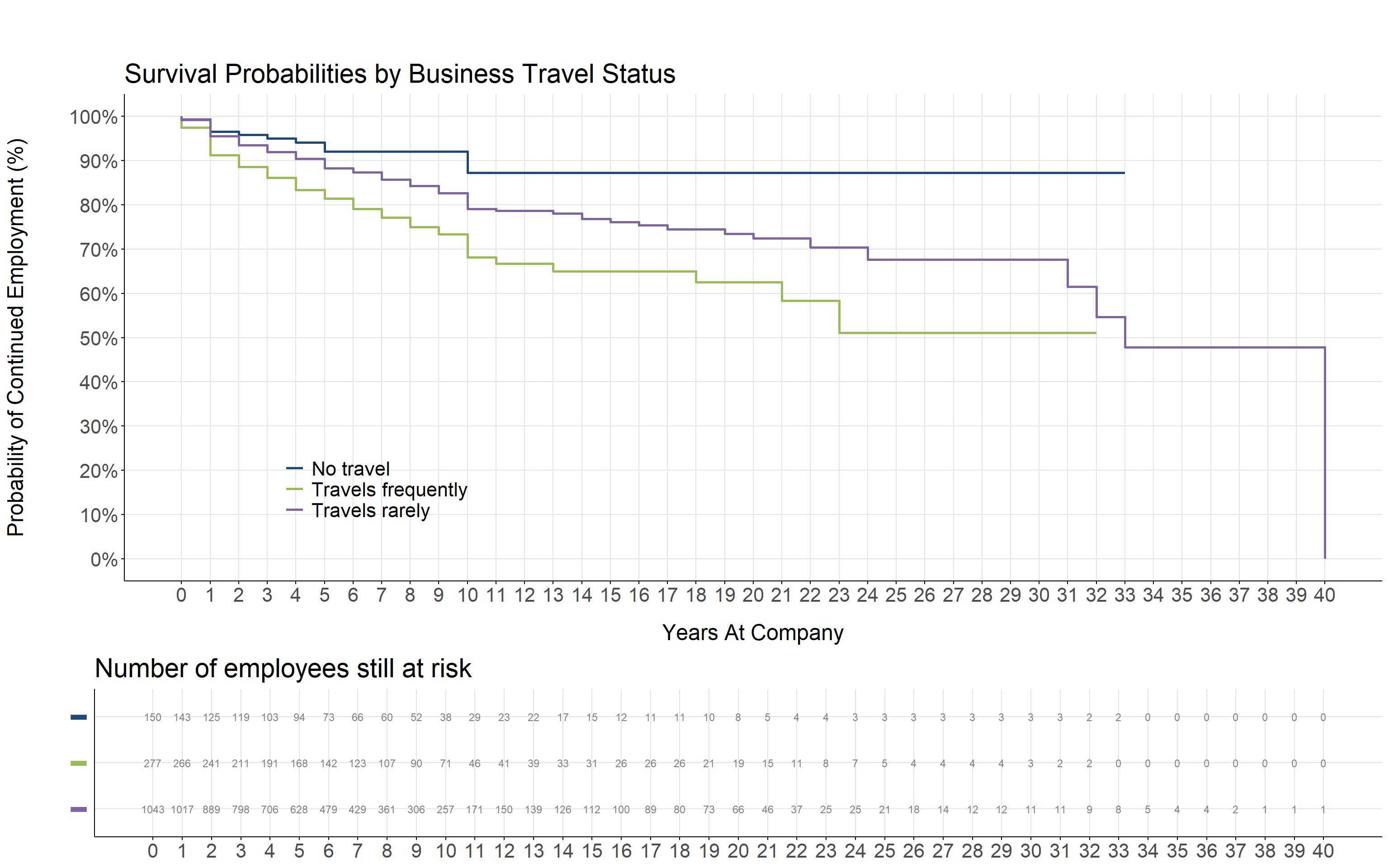
Employees who travel frequently show the lowest retention, with survival probability dropping to around 70% after 10 years. Those who do not travel maintain the highest retention, staying above 85% even after a decade. The separation between the curves can be seen from the early years.
Show the code
ggsurv_overtime <-
  ggsurvplot(fit = km_fit_OverTime,
            data = df,
            title = "\n\nSurvival Probabilities by Over Time Status",
            xlab = "Years At Company",
            ylab = "Probability of Continued Employment (%)\n",
            break.x.by=1,
            break.y.by=.1,
            conf.int = FALSE,
            censor = FALSE,
            xlim = c(0, max(df$YearsAtCompany)),
            surv.scale = "percent",
            risk.table = TRUE,
            risk.table.title = "Number of employees still at risk",
            risk.table.height = 0.22,
            risk.table.y.text = FALSE,
            fontsize = 3,
            legend.title = element_blank(),
            risk.table.col = "#808080",
            ggtheme = theme_survival,
            legend = c(0.2, 0.2),
            palette = c("#1F497D", "#9BBB59", "#8064A2", "#C0504D", "#4F81BD", "#F79646")
  )

ggsurv_overtime$table <- ggsurv_overtime$table + theme(axis.title.x = element_blank())
print(ggsurv_overtime)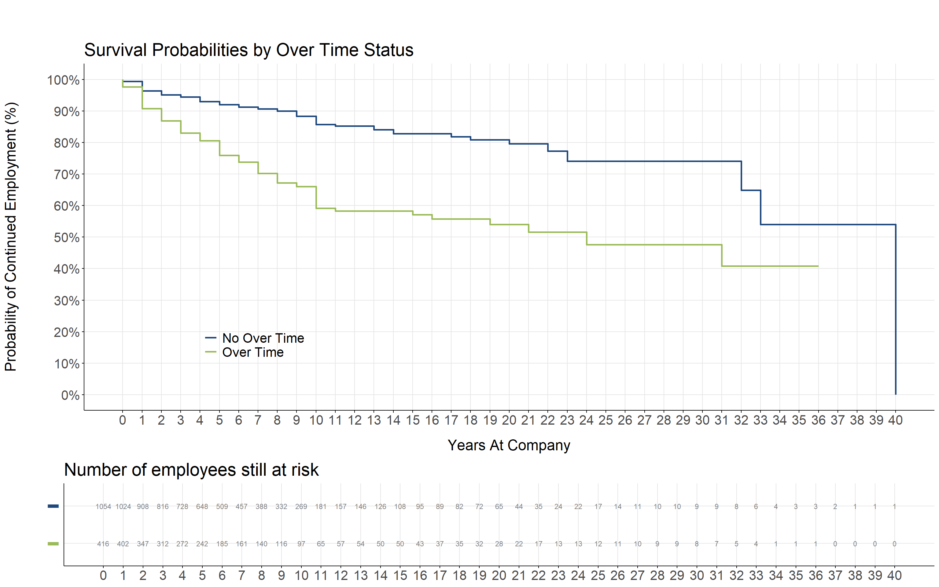
Employees who work overtime have a noticeably steeper decline in survival probability, falling to roughly 60% after 10 years, compared to about 85% for those who do not. The curves diverge within the first few years.
Show the code
ggsurv_combined <-
  ggsurvplot(fit = km_fit_BusinessTravel_OverTime,
            data = df,
            title = "\n\nSurvival Probabilities by Business Travel and Over Time Status",
            xlab = "Years At Company",
            ylab = "Probability of Continued Employment (%)\n",
            break.x.by=1,
            break.y.by=.1,
            conf.int = FALSE,
            censor = FALSE,
            xlim = c(0, max(df$YearsAtCompany)),
            surv.scale = "percent",
            risk.table = TRUE,
            risk.table.title = "Number of employees still at risk",
            risk.table.height = 0.35,
            risk.table.y.text = FALSE,
            fontsize = 3,
            legend.title = element_blank(),
            risk.table.col = "#808080",
            ggtheme = theme_survival,
            legend = c(0.2, 0.2),
            palette = c("#1F497D", "#9BBB59", "#8064A2", "#C0504D", "#4F81BD", "#F79646")
  )

ggsurv_combined$table <- ggsurv_combined$table + theme(axis.title.x = element_blank())
print(ggsurv_combined)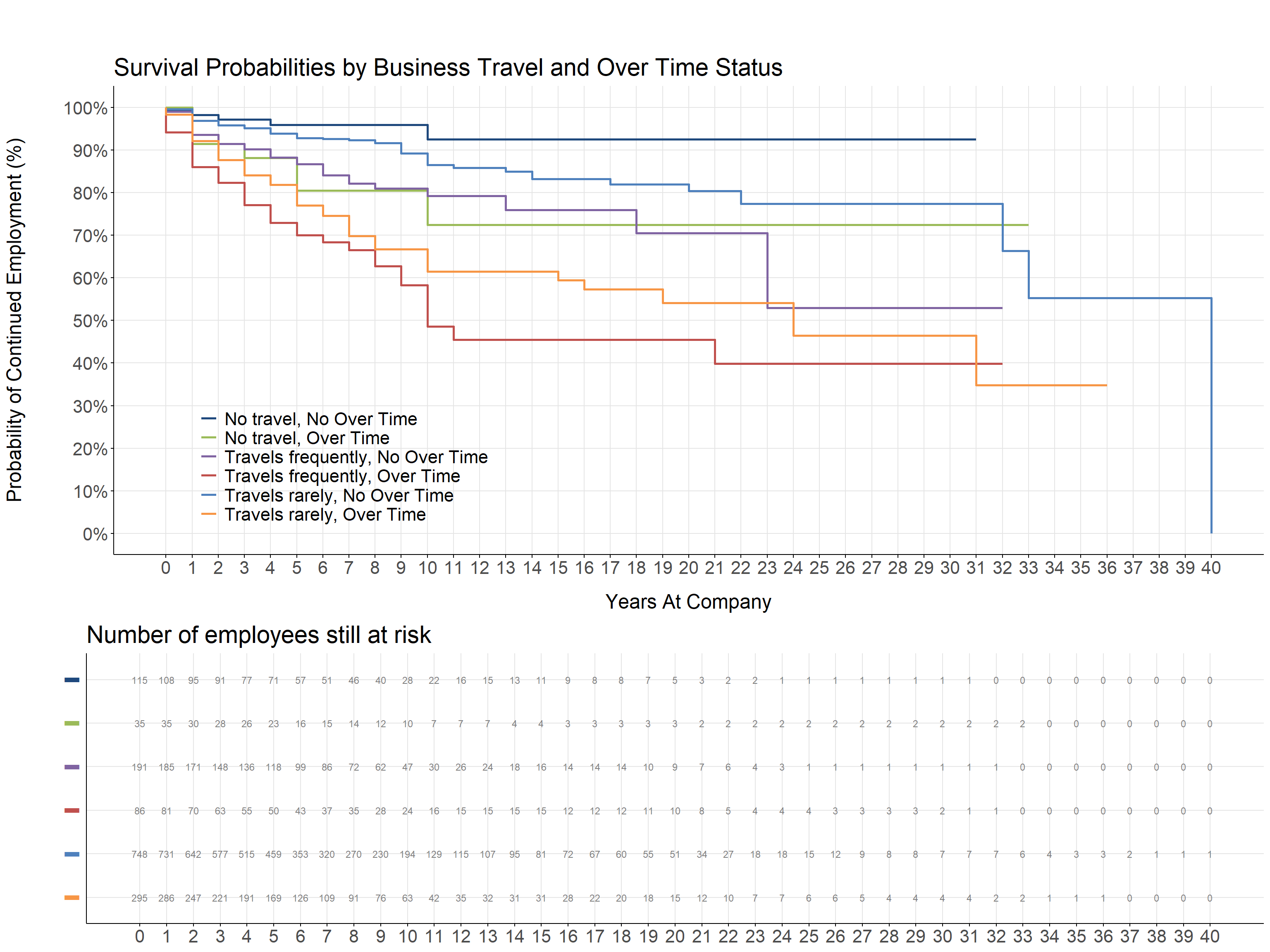
Combining the two variables shows that their effects compound. Frequent travelers who also work overtime have the lowest retention, with survival dropping below 50% by year 10. Meanwhile, non-traveling employees without overtime keep the highest retention rate, remaining above 90% through the same period. The difference between the groups becomes apparent almost immediately, with the gap widening over time.
Both of those groups are small, which the risk table under the chart makes visible: at year 10 they hold 24 and 28 employees. The two rarely-traveling groups, which carry most of the data, sit between the extremes with 61% and 87%.
Summary and further directions
These two posts covered the Kaplan-Meier method end to end: building a survival object, reading the curve, and splitting it by employee attributes. The same method is used for customer churn, equipment failure and clinical trials. One caution runs through all of it, and the risk tables under the charts are there to make it visible: once a group is down to a handful of employees, a single departure moves its curve, and conclusions drawn from that stretch carry far less weight than the ones drawn from the early years. The natural next step is the Cox proportional hazards model, which estimates the effect of each variable at the individual level instead of splitting the data into groups.